So, this post is supposed to function as my notes for the upcoming IEEE signal processing journal club presentation. I decided to pick the excellent paper by Batson, Spielman and Srivastava on Twice Ramanujan Sparsifiers. I can’t honestly even remember how I came across this paper, but it stuck in my mind as a really cool result that I wanted to understand one day. This seemed like as good a time as any to have a crack at it.
So Why Should I Care About This?
So the dumbest and most misleading summary I can give would be that for a given undirected graph, there is a sparse graph that contains almost the same information. The paper gives a constructive proof that such a sparse graph exists by giving a polynomial time complexity algorithm for finding this approximating graph. Neat! Only problem is that it is cubic in the number of vertices, which is exactly the same complexity order as the problem I was trying to avoid by using this result. Dang! Although there are other algorithms that do pretty much the same thing, such as this randomized algorithm that is linear in the number of edges of the graph. So as an utterly dirty applied mathematician I can use algorithms such as these and not feel too bad about it, since I now know that such good approximating graphs actually do exist.
A Motivating Example
I always find that a nice example from the everyday helps me understand why a particular result would be useful. So let’s imagine that you had wasted the last six years of your life trying to find things in laser scans. A completely hypothetical situation. One of the big problems you have with measuring stuff in the wild is that absolute position is hard to get accurately (say with an RTK GNSS system, accuracy in the order of cm), whereas relative position measurements are pretty straight forward and high accuracy (a time of flight laser pulse system, accuracy in the order of mm). It would be nice to be able to use all the measurements together to simultaneously map the world and locate yourself to get a better estimate of where everything is than from the individual measurements alone. This would mean you could make what is effectively a weighted average of all the different measurements to get a better accuracy.
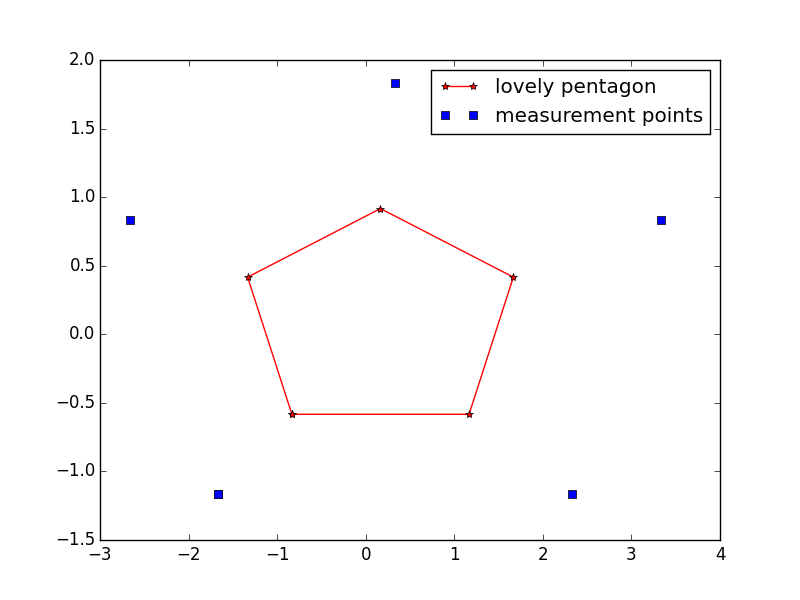
So let’s just pretend that you had a lovely pentagon that you wanted to measure, so you measured it from five positions around the outside with a terrestrial scanner, as represented in the following picture.

The set up is that the GNSS receiver on the scanner reports positions with a standard deviation of 5cm, and it measures the distance to the points of the pentagons with an accuracy of 5mm. Let’s go crazy and say that it also measures where the other measurement positions are as well with the same accuracy (say you left some markers on the ground that you can see with the scanner). Let’s also make it completely fake and say there are no attitude errors as well. The measurements from the range finder from the $i^{th}$ point to the $j^{th}$ point give the following equations.
i.e. you measure the distance between two points with the Lidar, and the position of a point with the GNSS system (with different levels of noise, we can lie to ourselves and say it is Gaussian to make our lives easier). Let’s make out lives even easier still and pretend we only care about the $z$ component of the position (generalizing this to all components is straight forward). Turning the usual crank of plugging into Bayes Theorem (with a few assumptions about priors) it can be shown that finding the $x$ that minimizes the following cost function will maximize the posterior probability of the question “where are all the points given the data”.
where $x$ is a vector of the $z$ position of all the measured points, $x_{0}$ is a vector of the GNSS measurements, $\lambda$ is a vector of regularization coefficients (zero for no GNSS measurement), $b$ is a vector where $b_i = \sum_{j=1}^nd_{ij}$ and (drum roll…) $A$ is the negative of the Graph Laplacian of the graph formed by considering the vertices of the graph as the positions to estimated and the presence of an edge indicates that a Lidar measurement between these two positions exist.
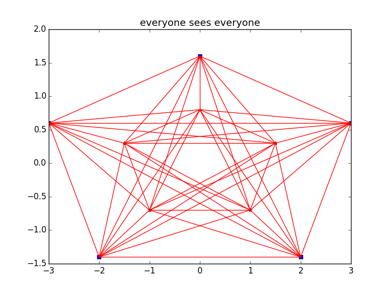
The awake amongst you notice that I have rigged the setup to give a complete graph here, 10 vertices too. Weird huh? It is a complete graph because every vertex is connected to every other vertex, as shown in the following picture.

Now this is all fine and dandy, we can solve this least squares problem with no issues at all. The question is what do we do when the problem gets freaking enormous, like the number of vertices is millions of feature point correspondences from thousands of poses in a large scale bundle adjustment problem? (Ignoring that the optimization problem is also non-linear now, let’s imagine we are worried about linear approximations in an Newton-Raphson type scheme). From here there are a few approaches, exploit the structure of $A$ to decompose the problem into more reasonable sub problems (such as the use of the Schur Complement in Bundle Adjustment solvers), solve a simpler system that approximates the original problem (a la “Sketching”) or design a really awesome preconditioner for an low memory iterative solution scheme like the conjugate gradient method (provided you can get $A$ to fit in memory at all). The results of the paper can help with the second and third approaches. I will give an outline of how is might work for the third approach.
Designing Preconditioners
So in general a preconditioner’s job is to apply a transformation to a linear system (such as the cost function above) to give a linear system whose condition number is much smaller than that of the original system, while being cheaper to calculate the original least squares problem. Since the condition number is smaller, the iterative scheme will converge much faster to a good approximate solution. This is where the spectral properties of Ramanujan Graphs become important. Note first that the condition number of a normal matrix is
i.e. the ratio of the absolute value of the largest and smallest eigenvalues of the matrix. Now note that the defining property of a Ramanujan Graph is that it is a d-regular graph (d edges per node) where the eigenvalues of the Graph Laplacian are between $d-2\sqrt{d-1}$ and $d+2\sqrt{d-1}$. Now the complete graph has $n$ for all it’s non-zero eigenvalues, so if we multiply all the edges of the Ramanujan Graph by $n/(d-2\sqrt{d-1}$ then we have the inequality that for all $x \in R^{V}$
where $G$ is the Complete Graph, $H$ is the Ramanujan Graph and
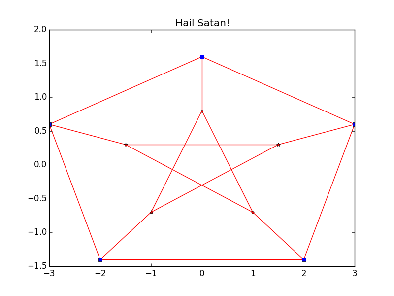
Joining all this together you can see that the Laplacian of the Ramanujan Graph acts as a good preconditioner to the Laplacian of the complete graph. Just for fun this is what the 3-regular Ramanujan Graph looks like for our 10 vertex complete graph.

This is fine if you have a complete graph, what do you do if you have an incomplete one, where measurements between all the points are not present? That is where this paper comes in where it that for any undirected graph $G$ it gives a method for constructing a graph $H$ with $d(n-1)$ edges such that
where now
which I think is pretty cool. The only problem is that the application I want it for is solving least squares problems and it has cubic complexity in the number of vertices. However, as stated in the introduction there are randomized algorithms with lower complexity, which is also very cool. Not sure that was a great explanation, please consult the papers linked for the words of people who know what they are talking about.
Anything Else?
Ramanujan Graphs are of interest in a whole bunch of fields as they are spectrally optimal expander graphs. This links in with things like designing robust networks, i.e. you can think of them as the “most connected” graphs of a fixed degree. This results in the generalization presented in the paper flowing over into these applications too, where it is unnatural to consider the complete graph as the graph to be approximated. As hinted at before graph sparsification also links in with the very interesting idea of “sketching”, finding a much smaller least squares problem to solve that gives almost the same solution. I don’t know much about this area but it is very intuitive, for most least squares problems you have much, much more data than you actually need to get a good solution. If only you could pick out the parts of your $A$ and $b$ that mattered in a systematic way.